Test package
Unite testing and numerical validation
Submodules
Test.test_Elasticity2D module
Numerical validation of the Elasticity2D Class
Tests
5 tests where made for validating the Elasticity2D class.
All of these 5 test are based in the same procedure. The objective is to compare the solution of the displacements profile in a cantilever beam.
Geometry
The input geometry has 400 elements, 10 in y direction, 40 in x directions. The input geometry file can be generated using TestGeometry class.
The beam geometrical properties are:
b = 0.3 m
h = 0.5 m
L = 2 m
E = 20000 KPa
\(\gamma=23.54\frac{kN}{m^3}\)
\(v=0.2\)
All tests are compared whit the analitycal solution of the beam deflections.
The results are obtained using the profile option of the package. The location of all profiles are in the centroid of the beam alog the y axis.
The Plane Stress formulation include shear effects. So, It is needed to obtain analytical solutions that includes such effects. The easyest way is to obtain the analytical solution using the virtual work statement.
Virtual work procedure for a cantilever beam
The virtual work statement is useful for calculate the dispacements in a given point. The displacements with felxion and shear effects can be calculated as:
where:
\(\hat{p}\) is point load applied in the place where the displacement want to be calculated. The load magnitude is 1.
\(\hat{M}\) is the moment diagram produced by the load \(\hat{p}\).
\(\hat{V}\) is the shear diagram produced by the load \(\hat{p}\).
For calculate the displacements in any point of the element lenght, the load \(\hat{p}\) have to be applied in a distance \(z\).

Moment and shear diagram for virtual load.
Since the diagrams are only different from 0 in length z, the virtual work statement can be rewritten as:
\(M\) and \(V\) are case dependent an these expresions will be developed for each test case.
- class Test.test_Elasticity2D.TestElasticity2D(methodName='runTest')
Bases:
TestCasePlane Stress tests 1. Uniform load applied as an uniform load in all elements. 2. Uniform load applied as a external load in the superior elements of the beam. 3. Point load applied in the beam lenght. The load is applied as a shear stress load. 4. Point load applied in the beam lenght. The load is applied as point load in the corner node. 5. Triangular load applied in the superior elements of the beam.
- test_cantilever_beam_point_1()
Test if the FEM solution matches the next analytical solution:
For the load condition, the moment an shear diagram can be described by the following equations:
\[M=PL\left(1-\frac{x}{L}\right)\]\[V=P\]Solving the virtual work statement, the analitycal displacement can be calculated as:
\[U = \frac{Px^2}{6EI}\left(3L-x\right)+\frac{Px}{kAG}\]
FEM solution compared whit analytical solution
- test_cantilever_beam_point_2()
Test if the FEM solution matches the next analytical solution:
For the load condition, the moment an shear diagram can be described by the following equations:
\[M=PL\left(1-\frac{x}{L}\right)\]\[V=P\]Solving the virtual work statement, the analitycal displacement can be calculated as:
\[U = \frac{Px^2}{6EI}\left(3L-x\right)+\frac{Px}{kAG}\]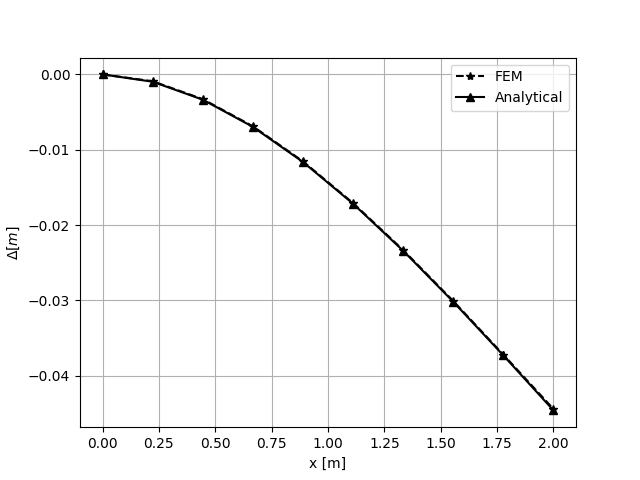
FEM solution compared whit analytical solution
- test_cantilever_beam_triangular_3()
Test if the FEM solution matches the next analytical solution:
For the load condition, the moment an shear diagram can be described by the following equations:
\[M=\frac{-WL^2}{6}+\frac{LW}{2}x-\frac{x}{2}\left(Wx\left(1-\frac{x}{L}\right)\right)-\frac{2}{3}x\left(\frac{Wx^2}{2L}\right)\]\[V=\frac{Wx^2}{2L}+Wx\left(1-\frac{x}{L}\right)-\frac{LW}{2}\]Solving the virtual work statement, the analitycal displacement can be calculated as:
\[U = \frac{Wx^2}{120LEI}\left(10L^3-10L^2x+5Lx^2-x^3\right)+\frac{Wx}{6kAGL}\left(x^2-3Lx+3L^2\right)\]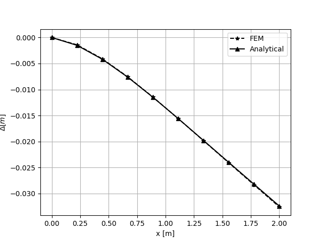
FEM solution compared whit analytical solution
- test_cantilever_beam_uniform_1()
Test if the FEM solution matches the next analytical solution:
For the load condition, the moment an shear diagram can be described by the following equations:
\[M=WLx-\frac{WL^2}{2}-\frac{Wx^2}{2}\]\[V=W(L-x)\]Solving the virtual work statement, the analitycal displacement can be calculated as:
\[U = \frac{Wx^2}{24EI}\left(x^2+6L^2-4Lx\right)+\frac{W}{kAG}\left(Lx-\frac{x^2}{2}\right)\]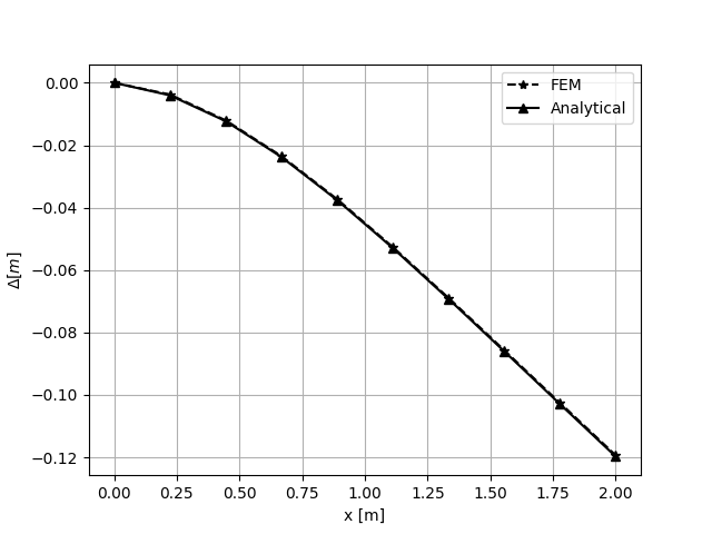
Test result: FEM solution compared whit analytical solution
- test_cantilever_beam_uniform_2()
Test if the FEM solution matches the next analytical solution:
For the load condition, the moment an shear diagram can be described by the following equations:
\[M=WLx-\frac{WL^2}{2}-\frac{Wx^2}{2}\]\[V=W(L-x)\]Solving the virtual work statement, the analitycal displacement can be calculated as:
\[U = \frac{Wx^2}{24EI}\left(x^2+6L^2-4Lx\right)+\frac{W}{kAG}\left(Lx-\frac{x^2}{2}\right)\]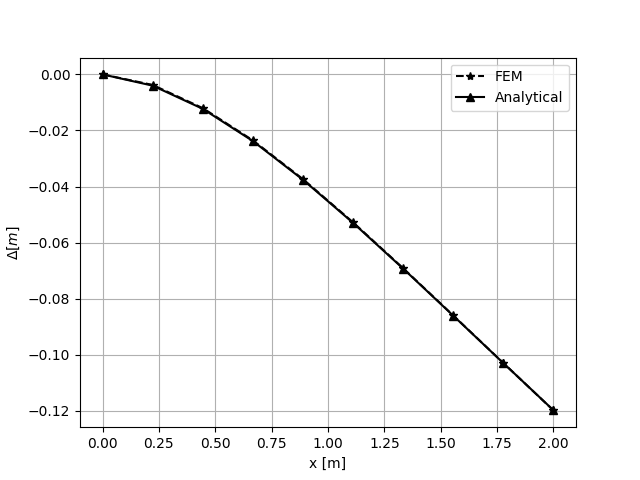
FEM solution compared whit analytical solution
Test.test_Elasticity3D module
Numerical validation of the Elasticity3D Class
Tests
1 tests where made for validating the Elasticity2D class.
All of these 1 test are based in the same procedure. The objective is to compare the solution of the displacements profile in a cantilever beam.
Geometry
The input geometry has 10000 elements.
The beam geometrical properties are:
b = 0.3 m
h = 0.6 m
L = 3.5 m
E = 21000 KPa
\(\gamma=23.54\frac{kN}{m^3}\)
\(v=0.2\)
All tests are compared whit the analitycal solution of the beam deflections.
The results are obtained using the profile option of the package. The location of all profiles are in the centroid of the beam alog the y axis.
The Plane Stress formulation include shear effects. So, It is needed to obtain analytical solutions that includes such effects. The easyest way is to obtain the analytical solution using the virtual work statement.
Virtual work procedure for a cantilever beam
The virtual work statement is useful for calculate the dispacements in a given point. The displacements with felxion and shear effects can be calculated as:
where:
\(\hat{p}\) is point load applied in the place where the displacement want to be calculated. The load magnitude is 1.
\(\hat{M}\) is the moment diagram produced by the load \(\hat{p}\).
\(\hat{V}\) is the shear diagram produced by the load \(\hat{p}\).
For calculate the displacements in any point of the element lenght, the load \(\hat{p}\) have to be applied in a distance \(z\).
Moment and shear diagram for virtual load.
Since the diagrams are only different from 0 in length z, the virtual work statement can be rewritten as:
\(M\) and \(V\) are case dependent an these expresions will be developed for each test case.
- class Test.test_Elasticity3D.TestElasticity3D(methodName='runTest')
Bases:
TestCasePlane Stress tests 1. Uniform load applied as an uniform load in all elements.
- test_cantilever_beam_uniform()
Test if the FEM solution matches the analytical solution:
For the load condition, the moment an shear diagram can be described by the following equations:
\[M=WLx-\frac{WL^2}{2}-\frac{Wx^2}{2}\]\[V=W(L-x)\]Solving the virtual work statement, the analitycal displacement can be calculated as:
\[U = \frac{Wx^2}{24EI}\left(x^2+6L^2-4Lx\right)+\frac{W}{kAG}\left(Lx-\frac{x^2}{2}\right)\]
Test result: FEM solution compared whit analytical solution
Test.test_Geometry module
Geometry tests
Test.test_Geometry2D module
Geometry tests
Test.test_Torsion2D module
Numerical validation of the Trosion2D Class
Tests
2 tests where made for validating the Torsion2D class. The objective of the test is to calculate the calculating polar moment of inertia (J) of a section.

Calculating polar moment of inertia (J)
Using the formulation of the Torsion2D class, the polar moment of inertia can be calculated as:
Where \(\Psi\) is the main variable solution of the Torsion2D class.
The integral can be computed by element using the following expresion:”
Where:
\(e\) is a single area element.
\(|Jac(\zeta_i)|\) is the determinant of the jacobian matrix.
\(U(\zeta_i)\) is the interpolated solution of the main variable.
\(\zeta_i\) is the Gauss-Legendre quadrature point.
\(W_i\) is the weight of the i-Gauss point.
\(N\) is the number of Gauss points.
\(n\) is the number of elements.
Hollow shapes
Due to the boundary conditions of the equation, it is not possible to introduce holes in the geometry. The holes can be modeled using elements affecting the shear modulus. The hole elements will have relatively close to zero shear modulus, while the material elements will have a higher shear modulus. In this case, a shear modulus of 80000 is used for material elements and a shear modulus of 1*10^-6 is used for hole elements.
A rotation angle of 1 is selected for all test cases.
- class Test.test_Torsion2D.TestTorsion2D(methodName='runTest')
Bases:
TestCaseTorsion2D Tests 1. Hollow circle. 2. Circle.
- test_inertia_circle()
Test if the polar moment of inertia (J) matches the analytical solution for circle. In this case, the analytical solutions is given by:
\[J = \frac{\pi}{2}\left(r^4\right)\]Where:
\(r\) is the radius.
- test_inertia_hollow_circle()
Test if the polar moment of inertia (J) matches the analytical solution for a hollow circle. In this case, the analytical solutions is given by:
\[J = \frac{\pi}{2}\left(r_1^4-r_2^4\right)\]Where:
\(r_1\) is the external radius.
\(r_2\) is the inner radius.