Examples package#
Examples index
Submodules#
Examples.EigenvaluesTest module#
Examples.EnmalladosTesis module#
Examples.ExampleD module#
Examples.ExampleE module#
Examples.ExampleF module#
Examples.ExampleGValidacion module#
Examples.Punto3 module#
Examples.Punto6 module#
Examples.TestsEigenvalues module#
Examples.a module#
AAAAAAAAAAAAAAAA TEST
Examples.b module#
Examples.example1 module#
Creation of 2D elements#
Coords and gdls (degrees of freedom) are given by a Numpy ndarray matrix.
In the coordinate matrix, each row represents a node of the element and each column a dimension. For example, a 2D triangular element of 3 nodes must have a 3x2 matrix.
In the gdls matrix, each row represents a variable of the node and each column a node. For example, a 2D triangular element of 3 nodes and 2 variables per node (plane stress) must have a 2x3 gdls matrix.
In this example several characteristics are tested:
The element creation and transformations are tested over 2 triangular (2D), 2 quadrilateral (2D) and 2 lineal (1D) elements.
The isBetwwen methods gives the oportunity to check if a given set of points is are inside a element.
The inverseMapping method allows to give a set of global coordinates and convert them to natural coordinates.
The jacobian graph allows to verigfy the numerical estability of the element
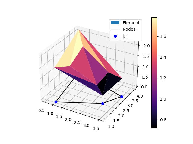
Coordinate trasformation and shape functions#
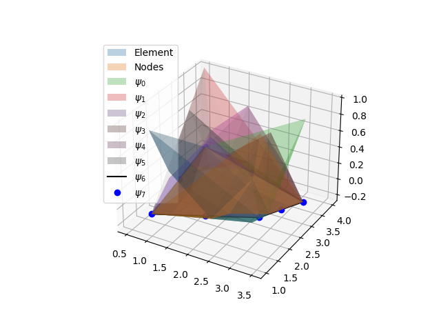
Serendipity (8 nodes 2D) element coordinate transformation and shape functions.#
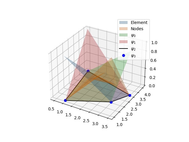
Quadrilateral (4 nodes 2D) element coordinate transformation and shape functions.#
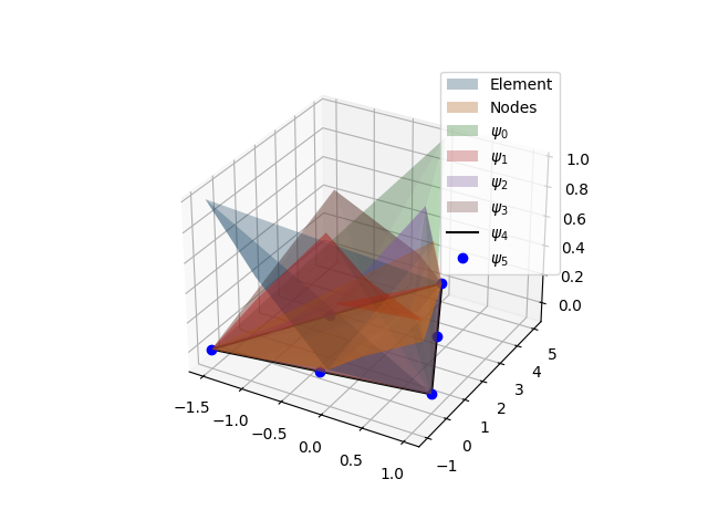
Triangular (6 nodes 2D) element coordinate transformation and shape functions.#
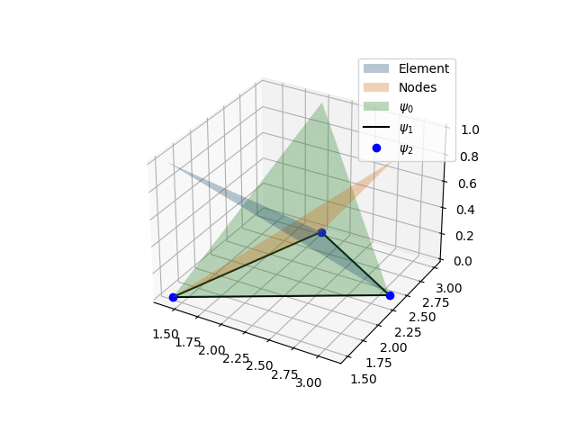
Triangular (3 nodes 2D) element coordinate transformation and shape functions.#
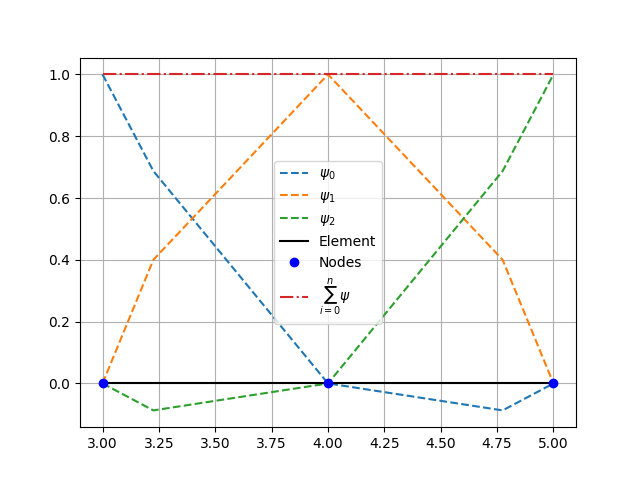
Line (3 nodes 1D) element coordinate transformation and shape functions.#
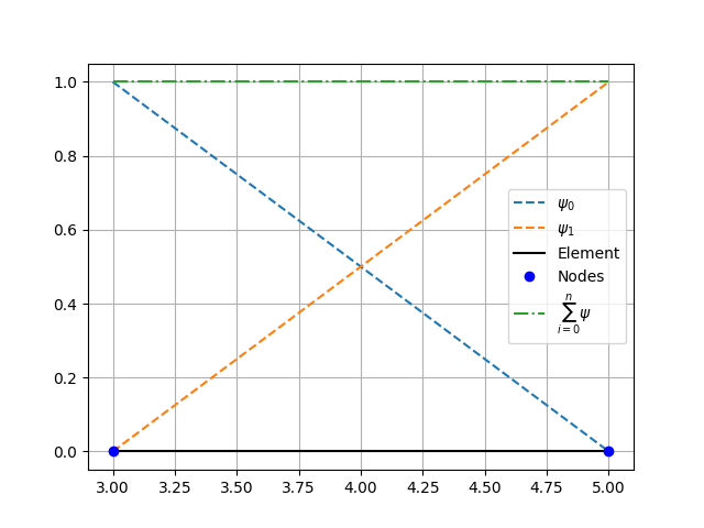
Line (2 nodes 2D) element coordinate transformation and shape functions.#
Point inside element (works in all dimensions)#
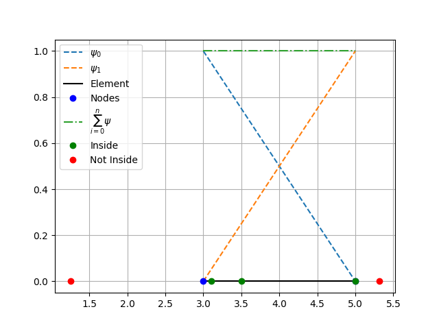
Test if given points are inside the element.#
Jacobian graphs#
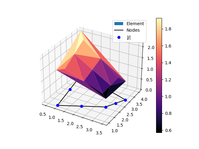
Serendipity (8 nodes 2D) element jacobian graph.#
Quadrilateral (4 nodes 2D) element jacobian graph.#
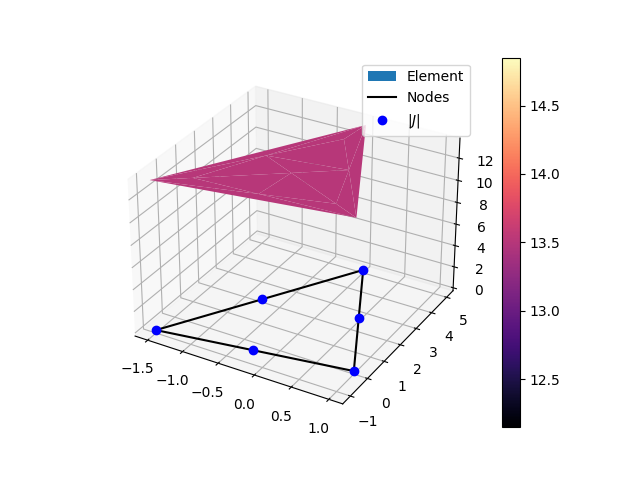
Triangular (6 nodes 2D) element jacobian graph.#
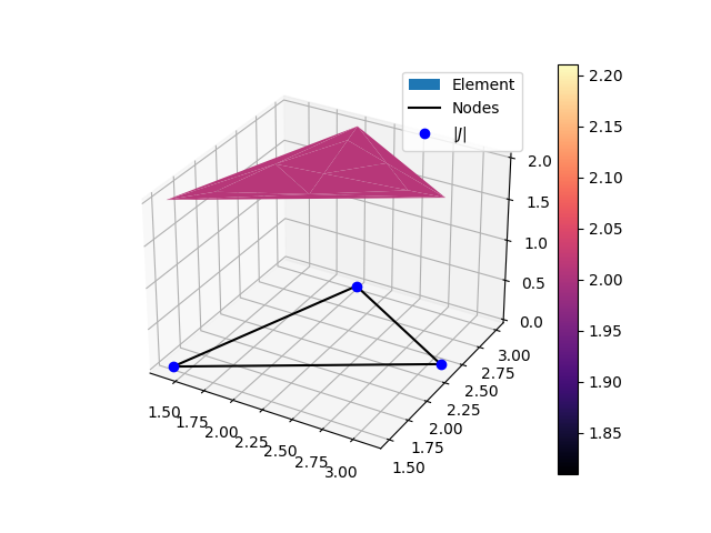
Triangular (3 nodes 2D) element jacobian graph.#
Code#
from FEM.Elements.E2D.Serendipity import Serendipity
from FEM.Elements.E2D.Quadrilateral import Quadrilateral
from FEM.Elements.E2D.LTriangular import LTriangular
from FEM.Elements.E2D.QTriangular import QTriangular

from FEM.Elements.E1D.LinealElement import LinealElement
from FEM.Elements.E1D.QuadraticElement import QuadraticElement

elements = []

coords = [[1, 1], [3, 2], [3.5, 3], [0.5, 4], [2, 1.5],
          [3.25, 2.5], [(3.5+.5)/2, 3.5], [(0.5+1)/2, 5/2]]
gdl = np.array([[1, 2, 3, 4, 5, 6, 7, 8]])
eRS = Serendipity(coords, gdl)
eRS2 = Serendipity(coords, gdl)
elements.append(eRS)

coords = [[1, 1], [3, 2], [3.5, 3], [0.5, 4]]
gdl = np.array([[1, 2, 3, 4]])
eRC = Quadrilateral(coords, gdl)
elements.append(eRC)

# [[-1.5, -1], [1, 0], [0, 5], [-0.25, -0.5], [0.5, 2.5], [-0.75, 2.0]]
coords = [[-1.5, -1], [1, 0], [0, 5]]
for i in range(len(coords)-1):
    coords += [[(coords[i][0]+coords[i+1][0])/2,
                (coords[i][1]+coords[i+1][1])/2]]
coords += [[(coords[i+1][0]+coords[0][0])/2,
            (coords[i+1][1]+coords[0][1])/2]]
gdl = np.array([[1, 2, 3, 4, 5, 6]])
eTC = QTriangular(coords, gdl)
elements.append(eTC)

coords = [[1.4, 1.5], [3.1, 2.4], [2, 3]]
gdl = np.array([[1, 2, 3]])
eTL = LTriangular(coords, gdl)
elements.append(eTL)

coords = [[3], [4], [5]]
gdl = np.array([[3, 4, 5]])
e = QuadraticElement(coords, gdl, 3)
elements.append(e)

coords = [[3], [5]]
gdl = np.array([[3, 5]])
e = LinealElement(coords, gdl, 3)
elements.append(e)

# Coordinate transformation
for i, e in enumerate(elements):
    e.draw()
    plt.show()

# Point inside element
p_test = np.array([1.25, 5.32, 3.1, 3.5, 5.0])
result = e.isInside(p_test)
e.draw()
plt.gca().plot(p_test[result], [0.0] *
               len(p_test[result]), 'o', c='g', label='Inside')
plt.gca().plot(p_test[np.invert(result)], [0.0] *
               len(p_test[np.invert(result)]), 'o', c='r', label='Not Inside')
plt.legend()
plt.legend()
plt.show()

# Inverse Mapping
z = eTL.inverseMapping(np.array([[1.3, 2.5, 3.5], [1.5, 2.6, 8.5]]))
# z = eTL.inverseMapping(np.array([[1.3],[1.5]]))
print(z)
# print(eTL.isInside(np.array([3.5,2.5])))

# Jacobian Graphs
for i, e in enumerate(elements):
    e.jacobianGraph()
    plt.show()
Examples.example10 module#
Examples.example11 module#
Examples.example13 module#
Examples.example14 module#
Examples.example15 module#
Examples.example16 module#
Examples.example17 module#
Examples.example18 module#
Examples.example19 module#
Examples.example2 module#
Geometry creation using triangles. Torsion2D#
An I shape section when a unitary rotation is applied.
The input mesh is created using the Delaunay class using second order elements.
Geomery#
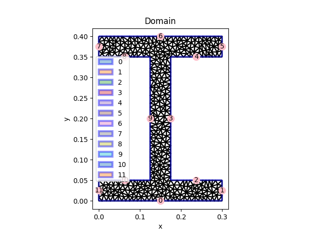
Input geometry created using Delaunay triangulations.#
Result#
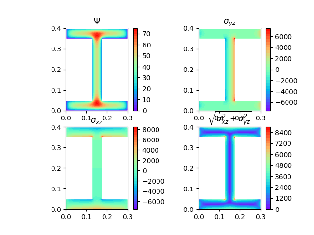
Analysis results.#
Code#
import matplotlib.pyplot as plt
from FEM.Torsion2D import Torsion2D
from FEM.Geometry import Delaunay, Geometry2D

a = 0.3
b = 0.3
tw = 0.05
tf = 0.05
E = 200000
v = 0.27
G = E / (2 * (1 + v))
phi = 1
# Geometry perimeter
vertices = [
    [0, 0],
    [a, 0],
    [a, tf],
    [a / 2 + tw / 2, tf],
    [a / 2 + tw / 2, tf + b],
    [a, tf + b],
    [a, 2 * tf + b],
    [0, 2 * tf + b],
    [0, tf + b],
    [a / 2 - tw / 2, tf + b],
    [a / 2 - tw / 2, tf],
    [0, tf],
]
# Input string to the delaunay triangulation.
# o=2 second order elements.
# a=0.00003 Maximum element area.
params = Delaunay._strdelaunay(constrained=True, delaunay=True,
                               a=0.00003, o=2)
# Mesh reation.
geometria = Delaunay(vertices, params)

# geometria.exportJSON('Examples/Mesh_tests/I_test.json') # Save the mesh to a file.
# geometria = Geometry2D.importJSON('Examples/Mesh_tests/I_test.json') # Load mesh from file.

# Show the geometry.
geometria.show()
plt.show()

# Create the Torsion2D analysis.
O = Torsion2D(geometria, G, phi)
O.solve() # All finite element steps.
plt.show()
Examples.example20 module#
Examples.example21 module#
Examples.example22 module#
Examples.example23 module#
Examples.example24 module#
Examples.example25 module#
Examples.example26 module#
Examples.example27 module#
Examples.example28 module#
Examples.example29 module#
Examples.example3 module#
Geometry creation using triangles. Torsion2D#
An square shape section when a unitary rotation is applied.
The input mesh is created using the Delaunay class using second order elements.
Geomery#
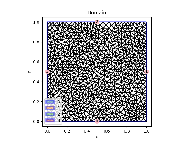
Input geometry created using Delaunay triangulations.#
Result#
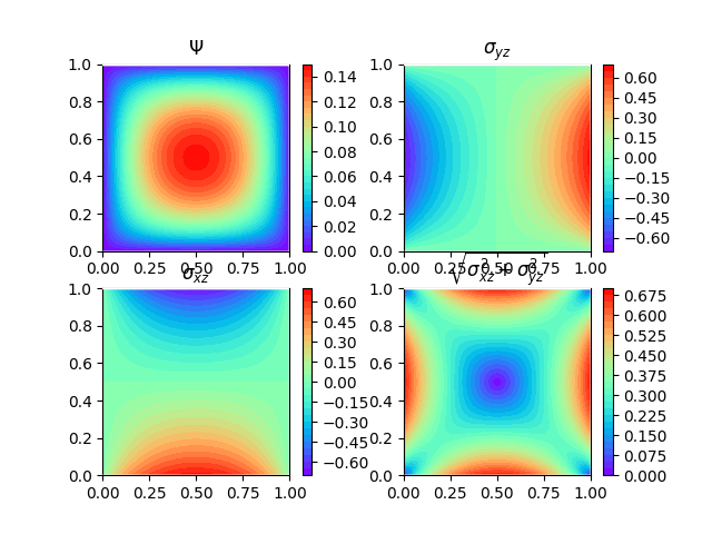
Analysis results.#
Code#
import matplotlib.pyplot as plt
from FEM.Torsion2D import Torsion2D
from FEM.Geometry import Geometry2D, Delaunay

a = 1
b = 1
E = 200000
v = 0.27
G = E/(2*(1+v))*0+1
phi = 1

# Use these lines to create the input geometry and file
# coords = np.array([[0, 0], [1, 0], [1, 1], [0, 1.0]])
# params = Delaunay._strdelaunay(a=0.0001, o=2)
# geo = Delaunay(coords, params)
# geo.exportJSON('Examples/Mesh_tests/Square_torsion.json')

geometria = Geometry2D.importJSON(
    'Examples/Mesh_tests/Square_torsion.json')
geometria.show()
plt.show()
O = Torsion2D(geometria, G, phi, verbose=True)
O.solve()
plt.show()
Examples.example30 module#
Examples.example31 module#
Examples.example32 module#
Examples.example33 module#
Examples.example34 module#
Examples.example35 module#
Examples.example36 module#
Examples.example37 module#
Examples.example39 module#
Examples.example4 module#
Ordinary diferential equation 1D#
The current file ust the general formulation of the EDO1D Class using custom function coeficients.
Geomery#
Result#
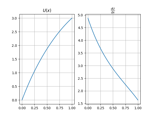
Analysis results.#
Code#
import matplotlib.pyplot as plt
from FEM.EDO1D import EDO1D
from FEM.Geometry import Lineal

# Define functions of the diferential equation
def a(x): return (x[0]**2-2)
def c(x): return (x[0]-3)
def f(x): return (x[0]**2-2)*6+(x[0]-3)*(3*x[0]**2)

# Define border conditions. List of border conditions. In the first node, value=0.0, in the last node, value = 3.0
cbe = [[0, 0.0], [-1, 3.0]]

lenght = 1
n = 500
o = 2
geometria = Lineal(lenght, n, o)
O = EDO1D(geometria, a, c, f)
O.cbe = cbe
O.solve()
plt.show()
Examples.example40 module#
Examples.example41 module#
Examples.example42 module#
Examples.example43 module#
Examples.example44 module#
Examples.example45 module#
Examples.example5 module#
Ordinary diferential equation 1D#
The current file ust the general formulation of the EDO1D Class using custom function coeficients.
Geomery#
Result#
Analysis results.#
Code#
import matplotlib.pyplot as plt
from FEM.EDO1D import EDO1D
from FEM.Geometry import Lineal

# Define functions of the diferential equation
def a(x): return (x[0]**2-2)
def c(x): return (x[0]-3)
def f(x): return (x[0]**2-2)*6+(x[0]-3)*(3*x[0]**2)

# Define border conditions. List of border conditions. In the first node, value=0.0, in the last node, value = 3.0
cbe = [[0, 0.0], [-1, 3.0]]

lenght = 1
n = 500
o = 2
geometria = Lineal(lenght, n, o)
O = EDO1D(geometria, a, c, f)
O.cbe = cbe
O.solve()
plt.show()